Gradient Descent
Gradient Descent is an iterative algorithm used to optimize objective functions, widely applied in machine learning and deep learning to train models by minimizing loss functions. It is recommended to first read the Machine Learning Basics article for background understanding.
Objective Function
Objective Function: Sometimes also called criterion, cost function, or loss function, is the function we aim to minimize, usually denoted as $J(\theta)$, where $\theta$ is the model parameter. For example, Mean Squared Error (MSE) used in linear regression is a common objective function.
Generally, we define $x^* = \arg\min_{x} J(x)$.
Derivative
Suppose we need to optimize the function $y = f(x)$, its derivative $f'(x)$ represents the rate of change at point $x$, or the slope of the tangent at that point.
Using the definition of the derivative, we see it indicates the trend of change at that point, helping us easily determine the direction of decrease.
Take a small positive number $\epsilon$, if $f'(x) > 0$, then $f(x - \epsilon) < f(x)$; otherwise, $f(x + \epsilon) < f(x)$. That is:
$$ f(x -\epsilon\cdot \text{sign}(f'(x))) < f(x) $$Therefore, the negative direction of the derivative is the direction of fastest decrease.
Gradient
Now, let’s extend the above process to multi-dimensional space. Suppose we have a multivariate function $f: \mathbb{R}^n \to \mathbb{R}$, with input as an $n$-dimensional vector $x = [x_1, x_2, \ldots, x_n]^T$ and output as a scalar $y = f(x)$. We want to find $x$ that minimizes $f(x)$.
In multi-dimensional space, the concept of derivative generalizes to the gradient. The gradient is a vector containing the partial derivatives with respect to each variable, denoted as:
$$ \nabla f(x) = \left[ \frac{\partial f}{\partial x_1}, \frac{\partial f}{\partial x_2}, \ldots, \frac{\partial f}{\partial x_n} \right]^T $$Each component $\frac{\partial f}{\partial x_i}$ represents the rate of change of $f$ with respect to $x_i$. The gradient vector points in the direction of the fastest increase at point $x$.
According to the conclusion from the derivative section, we might think to update along the direction of the partial derivatives. In fact, for a small positive $\epsilon$, the direction of fastest decrease for $f(x)$ is $-\nabla f(x)$, so:
$$ f(x - \epsilon \cdot \nabla f(x)) < f(x) $$Gradient Descent Algorithm
Based on the above, we can design an iterative algorithm to find the minimum of a function: at each step, move a small step in the negative direction of the derivative, gradually approaching the minimum.
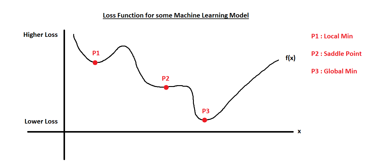
According to the properties of derivatives, points where $f'(x)=0$ are not necessarily minima. In practice, we rarely end up at saddle points due to floating-point errors. However, the minima we find may not be global minima, but rather local minima, which is usually acceptable since finding the global minimum is often infeasible and local minima are good enough.
For example, in the following figure, it is difficult to stop exactly at point P2 due to floating-point errors, but we are likely to stop at point P1, which, although not the global minimum, is usually sufficient.
Extending to multi-dimensional space, the gradient descent algorithm can be designed as follows:
- Initialize parameter $x$, either randomly or using a heuristic.
- Compute the gradient $\nabla f(x)$.
- Update parameter: $x = x - \alpha \cdot \nabla f(x)$, where $\alpha$ is the learning rate, controlling the step size.
- Repeat steps 2 and 3 until a stopping condition is met (e.g., gradient is small enough or maximum iterations reached).
Learning Rate
The learning rate $\alpha$ is an important hyperparameter in gradient descent, determining the step size for each update. Choosing an appropriate learning rate significantly affects convergence speed and final results.
- If the learning rate is too large, updates may overshoot the optimal solution or even cause divergence.
- If the learning rate is too small, convergence will be very slow, requiring many iterations and increasing computational cost. Usually, the learning rate is tuned experimentally, and techniques like learning rate decay can be used to adjust it dynamically for better convergence. These techniques are not discussed here.